Tutorial with Quantum ESPRESSO

Since the version 6.2, Quantum ESPRESSO can generate data-files for FermiSurfer. The following quantities can be displayed through FermiSurfer.

• The absolute value of the Fermi velocity \(|{\bf v}_{\rm F}|\) (fermi_velocity.x).

• The projection onto each atomic orbital \(|\langle \phi_{n l m} | \psi_{n k} \rangle|^2\) (fermi_proj.x)

Building PostProcess tool

For displaying the above quantities with FermiSurfer, we have to build PostProcess tools (tools for plotting the band structure, the charge density, etc.) in QuantumESPRESSO as follows:

$ make pp

SCF calculation

Now we will move on the tutorial. First, we perform the electronic-structure calculation with pw.x. We will treat MgB₂ in this tutorial. The input file is as follows.

scf.in

&CONTROL
 calculation = 'scf',
  pseudo_dir = './',
      prefix = 'mgb2' ,
      outdir = './'
/
&SYSTEM
       ibrav = 4,
   celldm(1) = 5.808563789,
   celldm(3) = 1.145173082,
         nat = 3,
        ntyp = 2,
     ecutwfc = 50.0 ,
     ecutrho = 500.0 ,
 occupations = 'tetrahedra_opt',
/
&ELECTRONS
/
ATOMIC_SPECIES
 Mg    24.3050   Mg.pbe-n-kjpaw_psl.0.3.0.upf
  B    10.811    B.pbe-n-kjpaw_psl.0.1.upf
ATOMIC_POSITIONS crystal
 Mg    0.000000000    0.000000000    0.000000000    
  B    0.333333333    0.666666667    0.500000000    
  B    0.666666667    0.333333333    0.500000000    
K_POINTS automatic 
16 16 12 0 0 0

Pseudopotentials used in this example are included in PS Library, and they can be downloaded from the following address:

• http://theossrv1.epfl.ch/uploads/Main/NoBackup/Mg.pbe-n-kjpaw_psl.0.3.0.upf

• http://theossrv1.epfl.ch/uploads/Main/NoBackup/B.pbe-n-kjpaw_psl.0.1.upf

We put the input file and the pseudopotential in the same directory, and run pw.x at that directory.

$ mpiexec -np 4 pw.x -npool 4 -in scf.in

the number of processes and the number of blocks for k-paralleliztion (npool) can be arbitlary numbers. We also can perform additional non-scf calcultion with a different k-grid.

Compute and display Fermi velocity

We run fermi_velocity.x program with the same input file as pw.x.

$ mpiexec -np 1 fermi_velocity.x -npool 1 -in scf.in

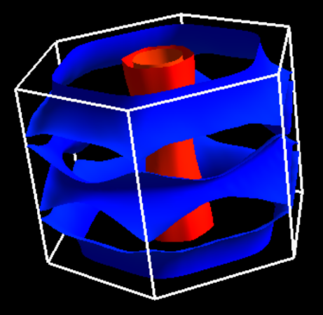
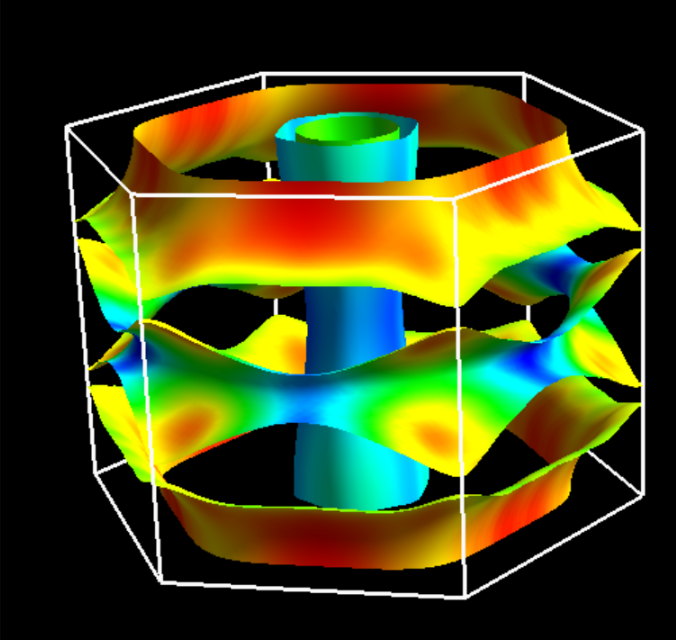
For this calculation, the number of blocks for k-paralleliztion (npool) should be 1 (or not specified). Then, the file for the Fermi velocity, vfermi.frmsf, is generated; this file can be read from FermiSurfer as

$ fermisurfer vfermi.frmsf

For the case of the collinear spin calculation, two files, vfermi1.frmsf and vfermi2.frmsf associated to each spin are generated.

Compute and display projection onto the atomic orbital

Then we will computeb the projection onto the atomic orbital. First we run projwfc.x with the following input file:

proj.in

&PROJWFC
   outdir = './'
    prefix='mgb2'
    Emin=-0.3422, 
    Emax=10.0578, 
    DeltaE=0.1
/
2
6 10

The input dates after the end of the name-list PROJWFC (/) is not used by projwfc.x. The number of processes and the number of blocks for the k-parallelization (npool) must to be the same as those for the execution of pw.x.

$ mpiexec -np 4 projwfc.x -npool 4 -in proj.in

excepting wf_collect=.true. in the input of pw.x.

the following description can be found in the beginning of the standard output of projwfc.x.

Atomic states used for projection
(read from pseudopotential files):

state #   1: atom   1 (Mg ), wfc  1 (l=0 m= 1)
state #   2: atom   1 (Mg ), wfc  2 (l=1 m= 1)
state #   3: atom   1 (Mg ), wfc  2 (l=1 m= 2)
state #   4: atom   1 (Mg ), wfc  2 (l=1 m= 3)
state #   5: atom   2 (B  ), wfc  1 (l=0 m= 1)
state #   6: atom   2 (B  ), wfc  2 (l=1 m= 1)
state #   7: atom   2 (B  ), wfc  2 (l=1 m= 2)
state #   8: atom   2 (B  ), wfc  2 (l=1 m= 3)
state #   9: atom   3 (B  ), wfc  1 (l=0 m= 1)
state #  10: atom   3 (B  ), wfc  2 (l=1 m= 1)
state #  11: atom   3 (B  ), wfc  2 (l=1 m= 2)
state #  12: atom   3 (B  ), wfc  2 (l=1 m= 3)

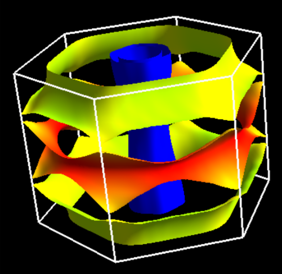
This indicates the relationship between the index of the atomic orbital (state #) and its character (for more details, please see INPUT_PROJWFC.html in QE). When we choose the projection onto the atomic orbital plotted on the Fermi surface, we use this index. For example, we run fermi_proj.x with above proj.in as an input file,

$ mpiexec -np 1 fermi_proj.x -npool 1 -in proj.in

and we obtain the data-file for FermiSurfer, proj.frmsf. In this case, after / in proj.in

2
6 10

we specify the total number of the displayed projection onto the atomic orbital as the first value (2) and projections to be summed as following indices. In this input, the sum of the 2pz of the first B atom (6) and the 2pz of the first B atom (10),

\[|\langle \phi_{B_1 2pz} | \psi_{nk} \rangle|^2 + |\langle \phi_{B_2 2pz} | \psi_{nk} \rangle|^2\]

is specified. We can display the Fermi surface as

$ fermisurfer proj.frmsf

If we want to plot the projections onto 2px and 2py orbitals of all B atoms, the input file for fermi_proj.x becomes

&PROJWFC
outdir = './'
prefix='mgb2'
Emin=-0.3422,
Emax=10.0578,
DeltaE=0.1
/
4
7 8 11 12

We do not have to run projwfc.x again.