Control FermiSurfer

Launch

For Linux, Unix, Mac

You can launch generated executable as follows:

$ fermisurfer mgb2_vfz.fs

You need a space between the command and input-file name. (The sample input file mgb2_vfz.fs contains \(z\) element of the Fermi velocity in MgB₂.)

For Windows

Click mouse right button on the input file. Choose “Open With …” menu, then choose fermisurfer.exe.

Then, Operations are printed, and Fermi surfaces are drawn (Fig. 1).

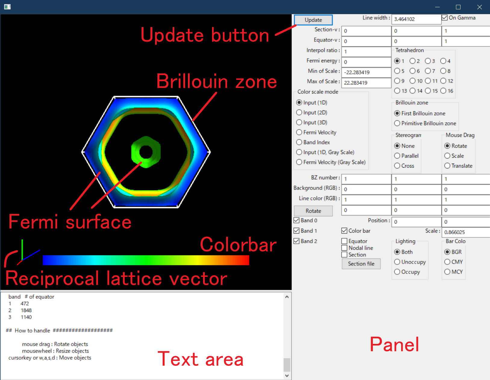
Main view.

The following operations are available:

• Rotation of objects with mouse drag

• Expand and shrink with mouse wheel

• Window re-sizing

• Moving objects with cursor keys (wasd for Windows). Also we can shift objects with double click.

• Opeerate by using the panel

Here, we can see all menus.

Note

Some operations are not applied immidiately, and after th “Update” button is pushed they are applied. Such operations are refered as “Update required”.

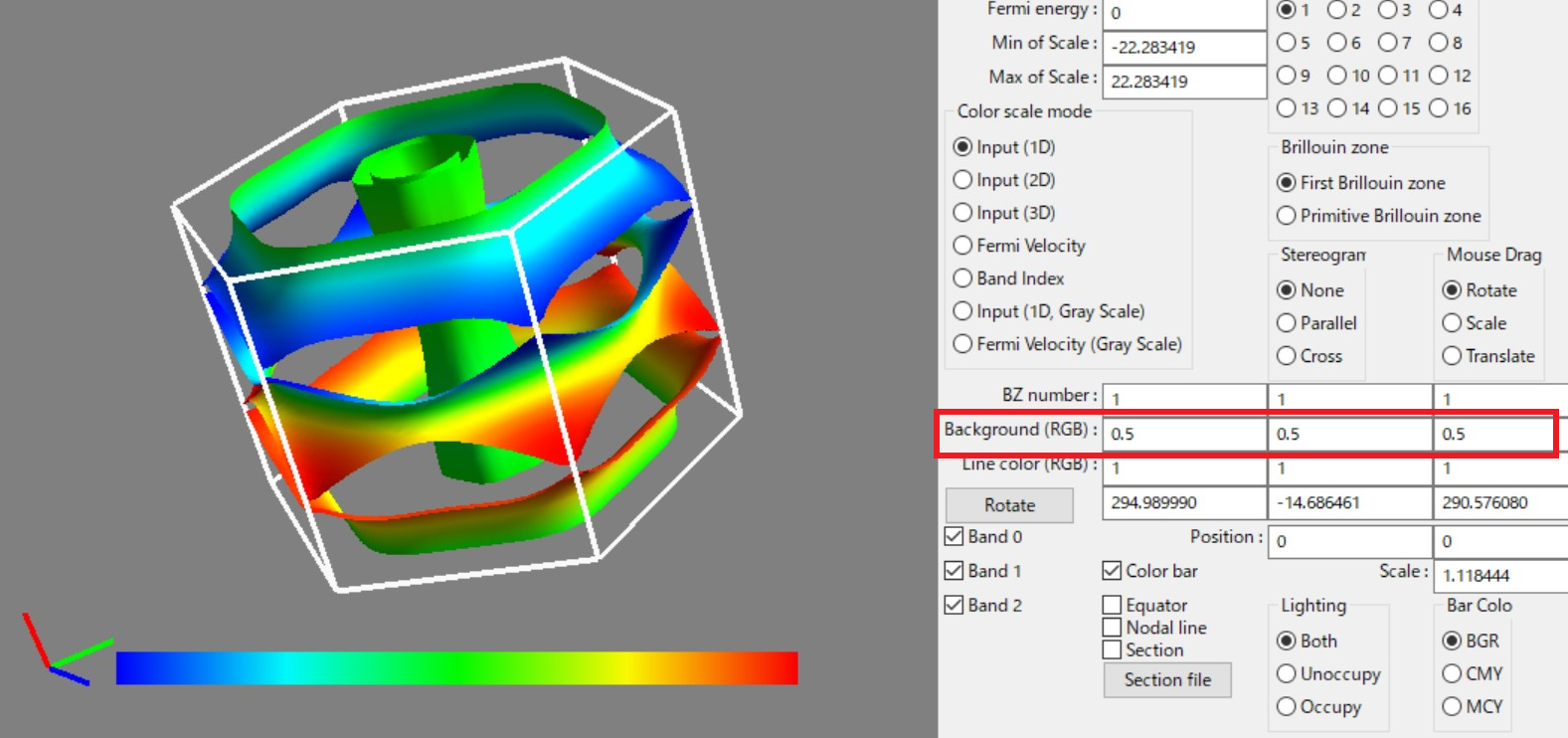
Background color

Background (RGB) : The background color is specified as RGB.

Line width

Line width : Modify the width of the Brillouin-zone boundary, the nodal line, etc.

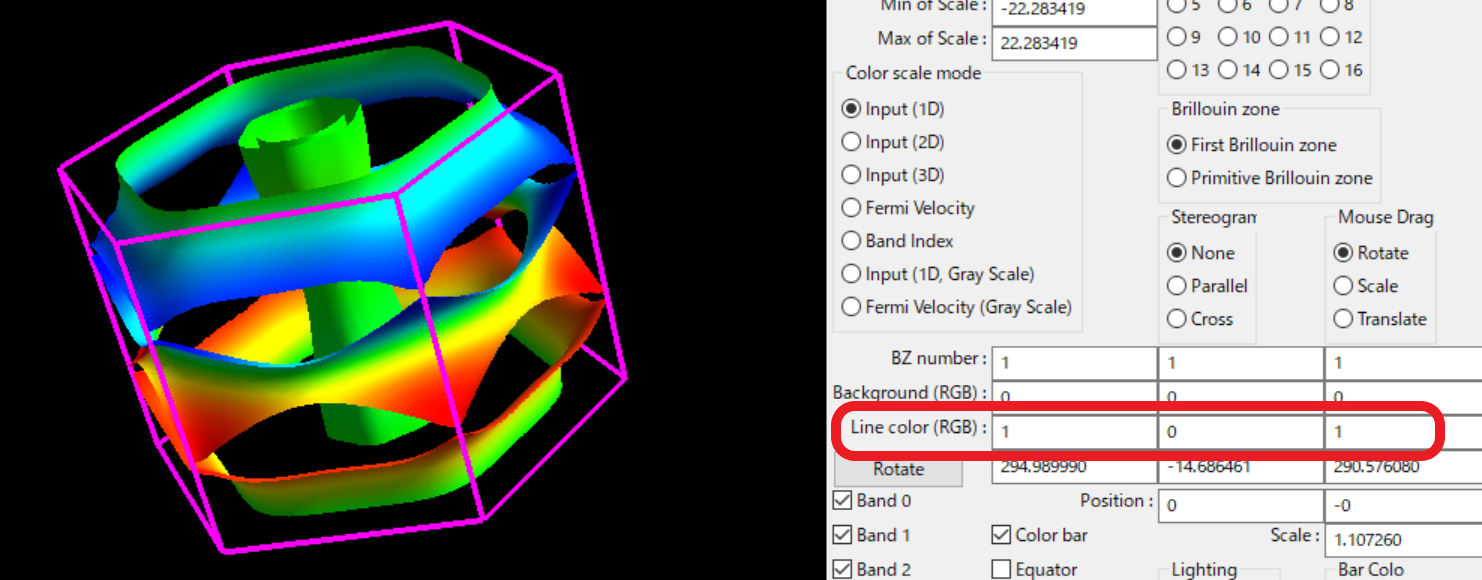
Line color

Line color (RGB) : The line color is specified with RGB.

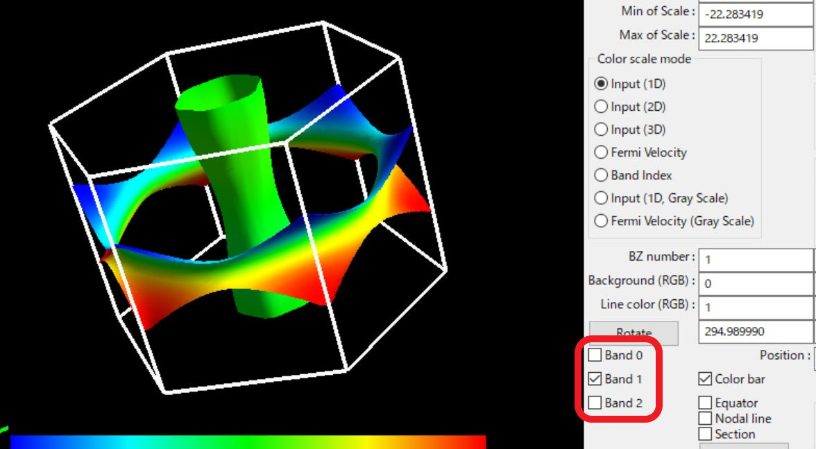
Band

Band 0, RGB, Band 1, RGB … : It makes each band enable/disable (Fig. 4).

Brillouin zone (Update required)

Brillouin zone : We choose Brillouin-zone type as follows (Fig. 5):

First Brillouin Zone

The region surrounded by Bragg’s planes the nearest to \({\rm \Gamma}\) point.

Primitive Brillouin Zone

A hexahedron whose corner is the reciprocal lattice point.

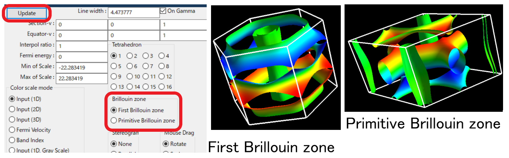
You can change the type of the Brillouin zone with “Brillouin zone” menu.

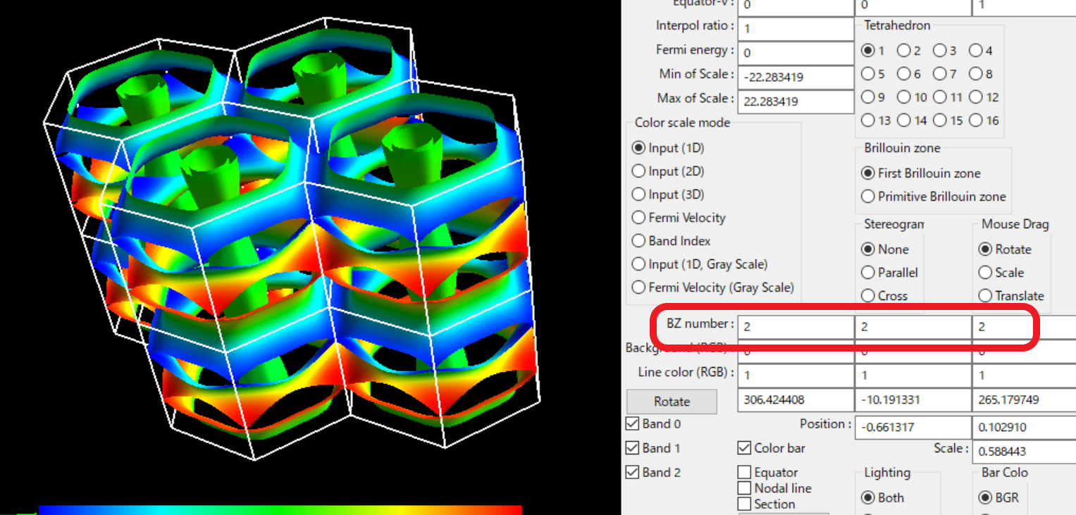
Number of Brillouin zone (Update required)

BZ number : We can specify how many zones are displayed along each reciprocal lattice vector.

Color bar

Color bar : The color bar becomes enable/disable (Fig. 7).

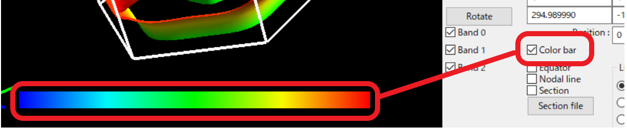
Toggling the color bar with “Color bar On/Off” menu.

Color scale mode (Update required)

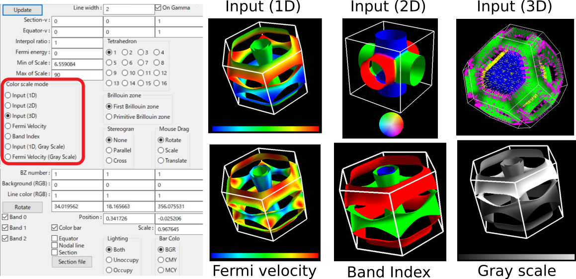
Color scale mode : It turns color pattern on Fermi surfaces (Fig. 8).

Input (1D) (default for the single input quatity) :

It makes blue as the minimum on Fermi surfaces and red as the maximum on them.

Input (2D) (default for the double input quatity) :

The color plot is shown with the color circle (see the figure).

Input (3D) (default for the triple input quatity) :

The input value is shown as arrows (thin triangles) on the Fermi surfaces. The color of the Fermi surfaces are the same sa “Band Index” case.

Fermi velocity (default for no input quantity)

Compute the Fermi velocity \({\bf v}_{\rm F} = \nabla_k \varepsilon_k\) with the numerical differentiation of the energy, and plot the absolute value of that.

Band Index :

Fermi surfaces of each band are depicted with uni-color without relation to the matrix element.

Input (1D, Gray), Fermi Velocity (Gray) :

Plot with gray scale.

Min of Scale, Max of Scale : We can change the range of the color plot by inputting into the text boxes. For 3D arrow plot the length of arrows can be changed by Max of Scale.

3D arrow step : Change the interval to display arrows at “Input (3D)” mode. Larger number indicates fewer arrows.

Arrow width : Change the thickness of arrow (triangle) at “Input (3D)” mode.

“Color scale mode” menu.

Perspective

Perspective : Turn on/off the perspective view.

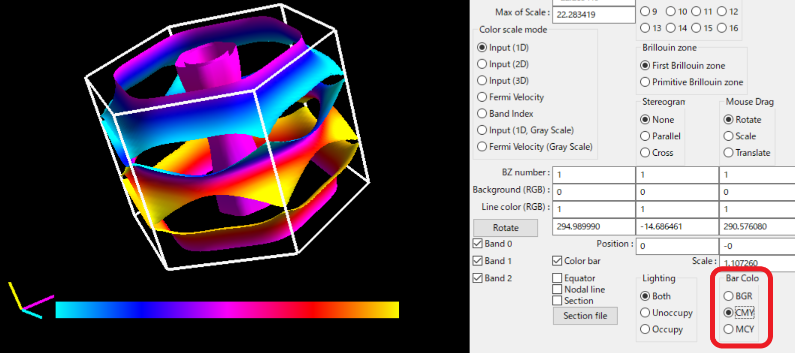
Color sequence for plot

Bar Color : We can specify the sequence of color plot. “BGR” is Blue-Cyan-Green-Yellow-Red, “CMY” is Cyan-Blue-Magenta-Red-Yellow, “MCY” is Magenta-Blue-Cyan-Green-Yellow.

Equator (Update required)

We can draw the line where \({\bf v}_{\rm F} \cdot {\bf k} = 0\) for a vector \({\bf k}\). See fig. 10. When it was created, Kawamura missunderstood that this coinsides the extremul orbit in dHvA (it is not true!). Maybe it is related to the ultrasonic attenuation.

Equator : We can toggle equator. This operation does not require the update.

Equator-v : Modify the direction of the tangent vector \({\bf k}\) (fractional coordinate). We need to push Update to reflect the change.

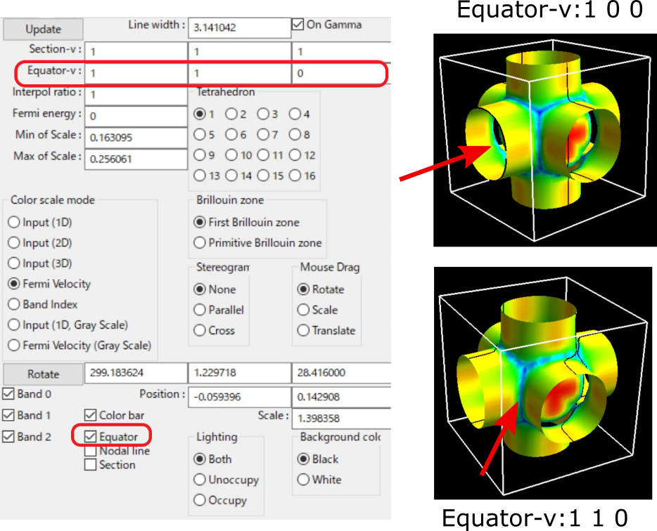
Display the equator with the “Equator” menu.

Interpolation (Update required)

Interpol ratio : Smooth the Fermi surface with the interpolation (Fig. 11). The time for the plot increases with the interpolation ratio.

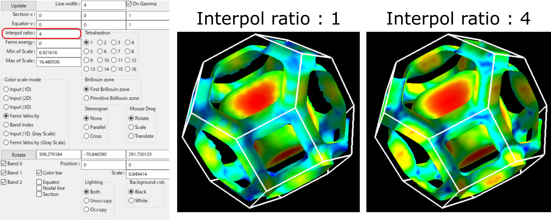
Modify the number of interpolation points from 1 to 4 with “Interpolate” menu.

Which (or both) side of Fermi surface is illuminated

Lighting : We can choose the illuminatedside of the Fermi surface (Fig. 12).

Both :

Light both sides.

Unoccupy :

Light unoccupied side.

Occupy :

Light the occupied side.

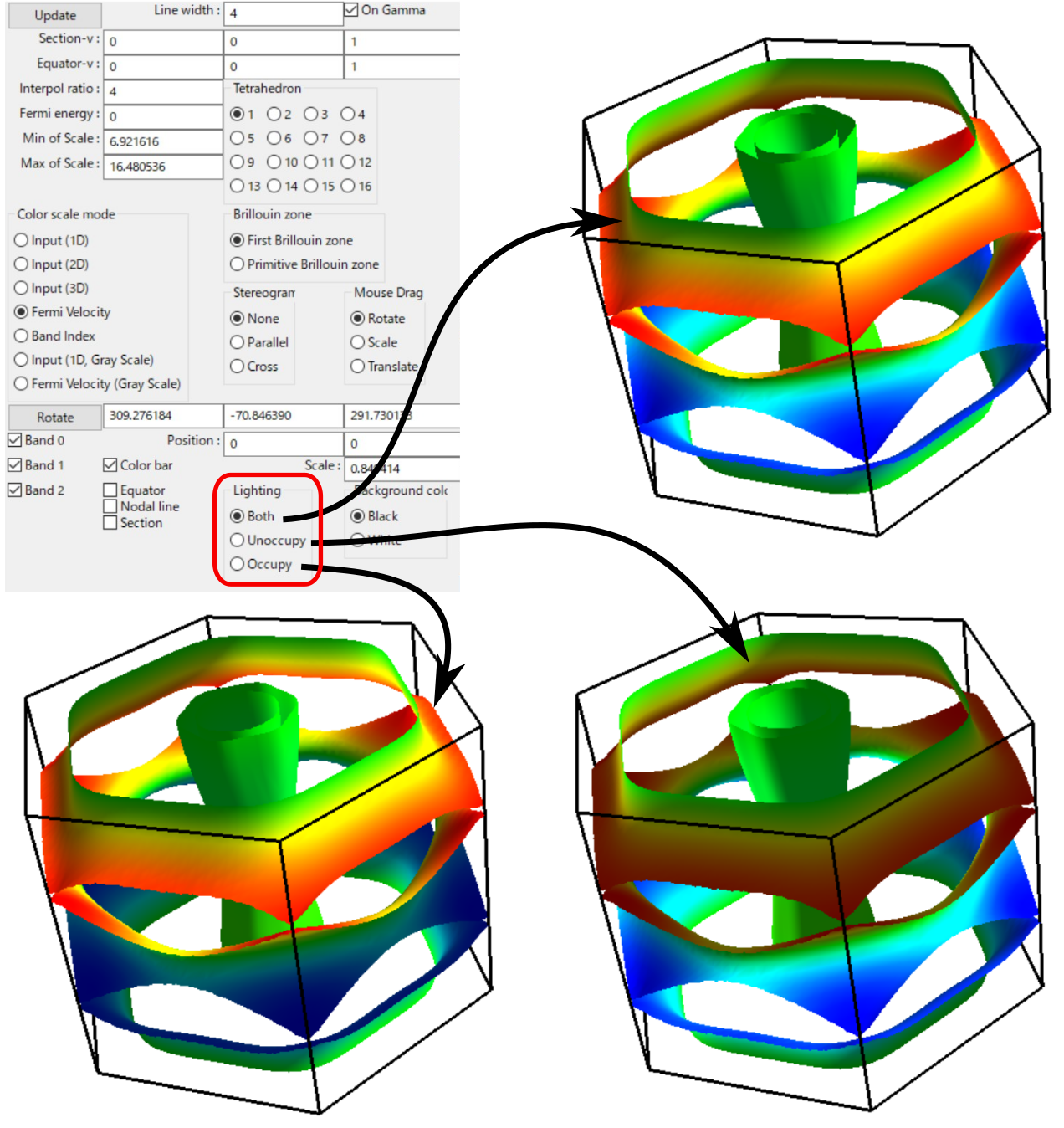
Change the lighted side by using the “Lighting” menu.

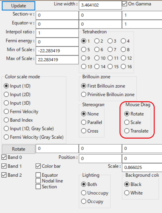
Mouse Drag

Mouse Drag : It turns the event of the mouse-left-drag.

Rotate(default)

Rotate the figure along the mouse drag.

Scale

Expand/shrink the figure in upward/downward drag.

Translate

Translate the figure along the mouse drag.

Nodal line

Nodal Line : The line on which the matrix element becomes 0 (we call it nodal line) becomes enable/disable (Fig. 14).

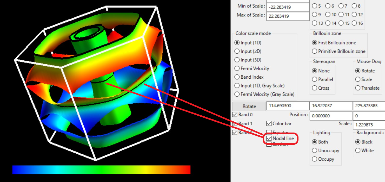
Toggling the node line with “Nodal line” menu.

Section of the Brillouine zone (Update required)

Display a 2D plot of the Fermi surface (line) on an arbitrary section of the Brillouin zone (Fig. 15).

Section : We can toggle it with the checkbox (this operation does not require update).

Section-v : We can change the normal vector with the textbox (fractional coordinate).

On Gamma If the it is turned on, the section crosses \(\Gamma\) point.

Section (RGB) : Change the color of plane representing the section in BZ.

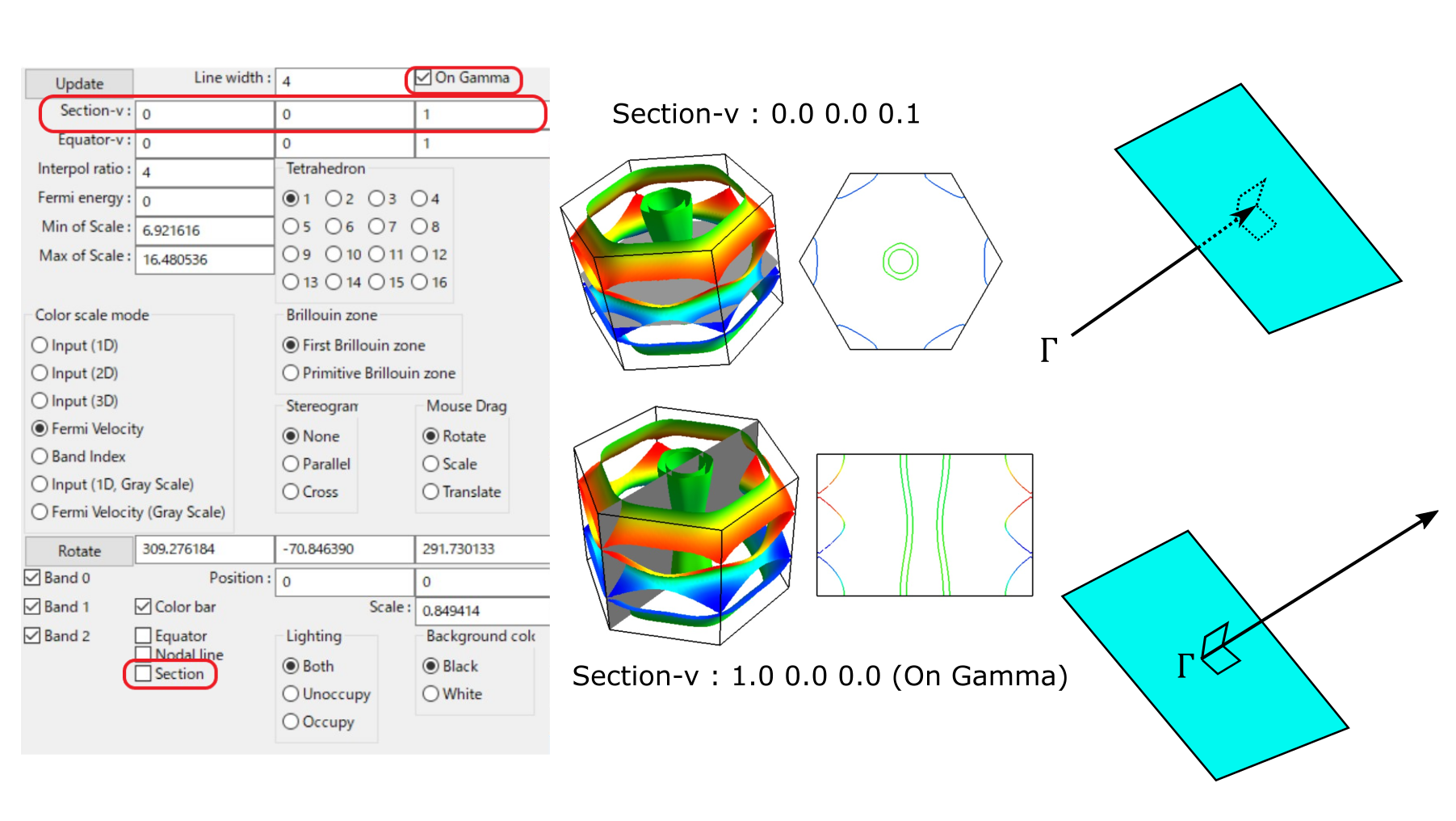
Display 2D plot of the Fermi surface (line) with “Section” menu.

Output section of the Brillouine zone

Section file : Above section of the Brillouin zone and Fermi surfaces are outputted into files “fermi_line.dat” and “bz_line.dat” by pushing this button.

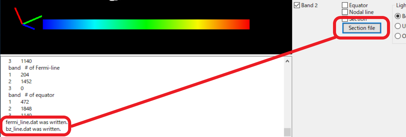
These files are plotted in gnuplot as follows:

plot "fermi_line.dat" w l, "bz_line.dat" w l

Shift Fermi energy (Update required)

Fermi energy : It shifts the Fermi energy (= 0 in default) to arbitrary value (Fig. 17).

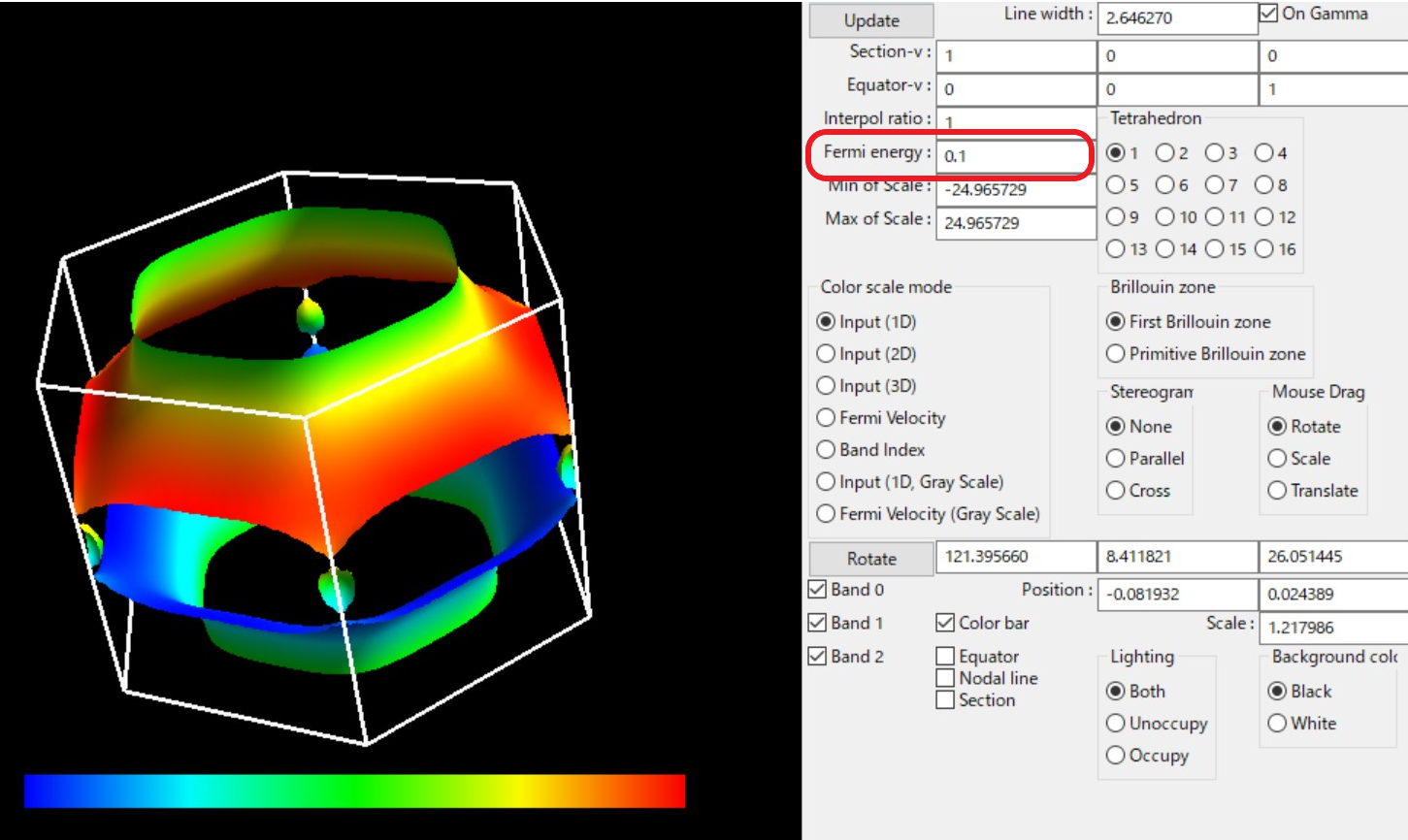
The Fermi energy is set from 0 Ry to 0.1 Ry with “Shift Fermi energy” menu

Stereogram

Stereogram : The stereogram (parallel eyes and cross eyes) becomes enabled/disabled (Fig. 18).

None (Default)

Parallel

Parallel-eyes stereogram

Cross

Cross-eyes stereogram

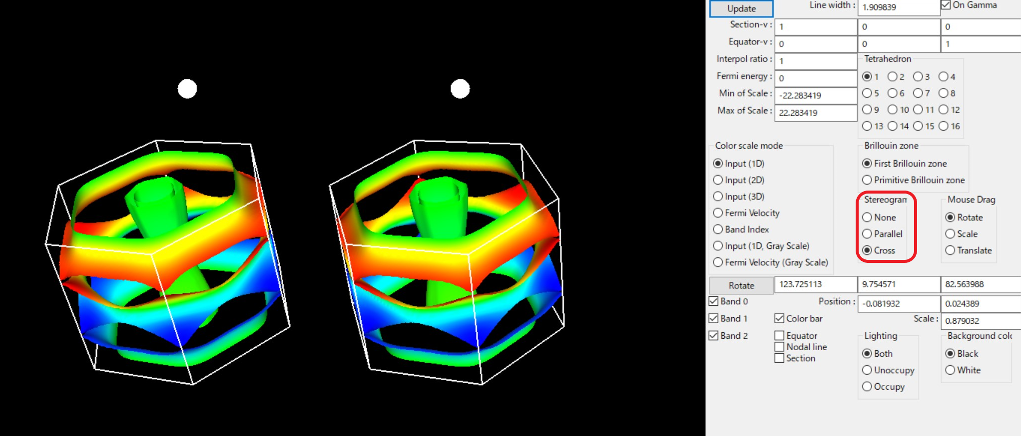
The stereogram becomes enabled/disabled with “Stereogram” menu.

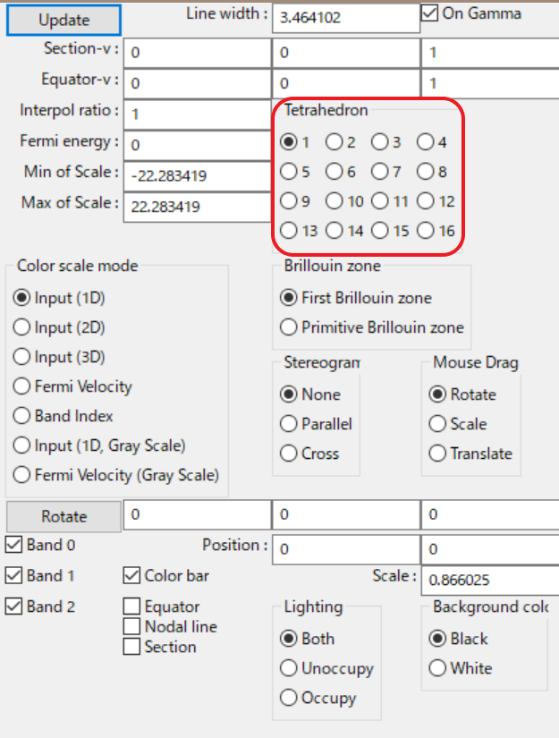
Tetrahedron (Update required)

Tetraghedron : You change the scheme to divide into tetrahedra (tetra # 1 as default). It is experimental.

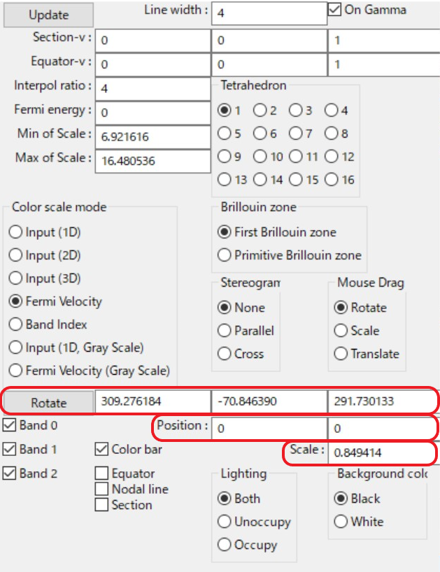
View point

Changing the view point.

Scale :

Change the size of the figure.

Position :

Change the xy position of the figure.

Rotate :

Change angles at x-, y-, z- axis. Rotations are performed as z-y-x axis if the “Roate” buttone is pushed.

In each menu, first the current value is printed. then a prompt to input the new value appears (Fig. 20).

Modify the view point by using “View point” menu

Arrow

Show an arrow (thin triangle) at arbitrary place. The following are specified in the fractional coordinate.

Arrow (Start) : Starting point

Arrow (End) : End point

Arrow (Diff) : Difference of above. Arrow (End) and Arrow (Diff) affects each other.

Arrow width : Modify the thickness of arrow (triangle).

Wireframe sphere

Show a wireframe sphere at arbitrary place. This is utilized together with HiLAPW. The following are specified in the Cartesian coordinate.

Sphere center : Center of sphere.

Sphere radius : Radius of sphere.

Nesting function

The following two kinds of nesting function are computed and written into a file readable by FermiSurfer.

delta*delta : File name is “doubledelta.frmsf”

\[\sum_{n n' \textbf{k}} \delta(\varepsilon_{n \textbf{k}}-\varepsilon_\textrm{F}) \delta(\varepsilon_{n' \textbf{k}+\textbf{q}}-\varepsilon_\textrm{F})\]

Lindhard : File name is “lindhard.frmsf”

\[-\sum_{n n' \textbf{k}} \frac{\theta(\varepsilon_\textrm{F} - \varepsilon_{n' \textbf{k}+\textbf{q}}) -\theta(\varepsilon_\textrm{F}-\varepsilon_{n \textbf{k}})} {\varepsilon_{n' \textbf{k}+\textbf{q}} - \varepsilon_{n \textbf{k}}}\]

Saving images

fermisurfer does not have any functions to save images to a file. Please use the screenshot on your PC.